Forecasting rate limits in claumon

June 2026 · Updated September 8, 2026 · Go · MIT-licensed

claumon is a local dashboard for Claude Code, shipped as a single binary with zero configuration required. Alongside live rate-limit gauges, session costs, and historical trends, it includes process controls and a memory-file browser with health checks, a relationship graph, and recoverable deletion. A companion VS Code extension brings usage and the dashboard into the editor. This page covers one piece: the forecaster behind the rate-limit gauges.

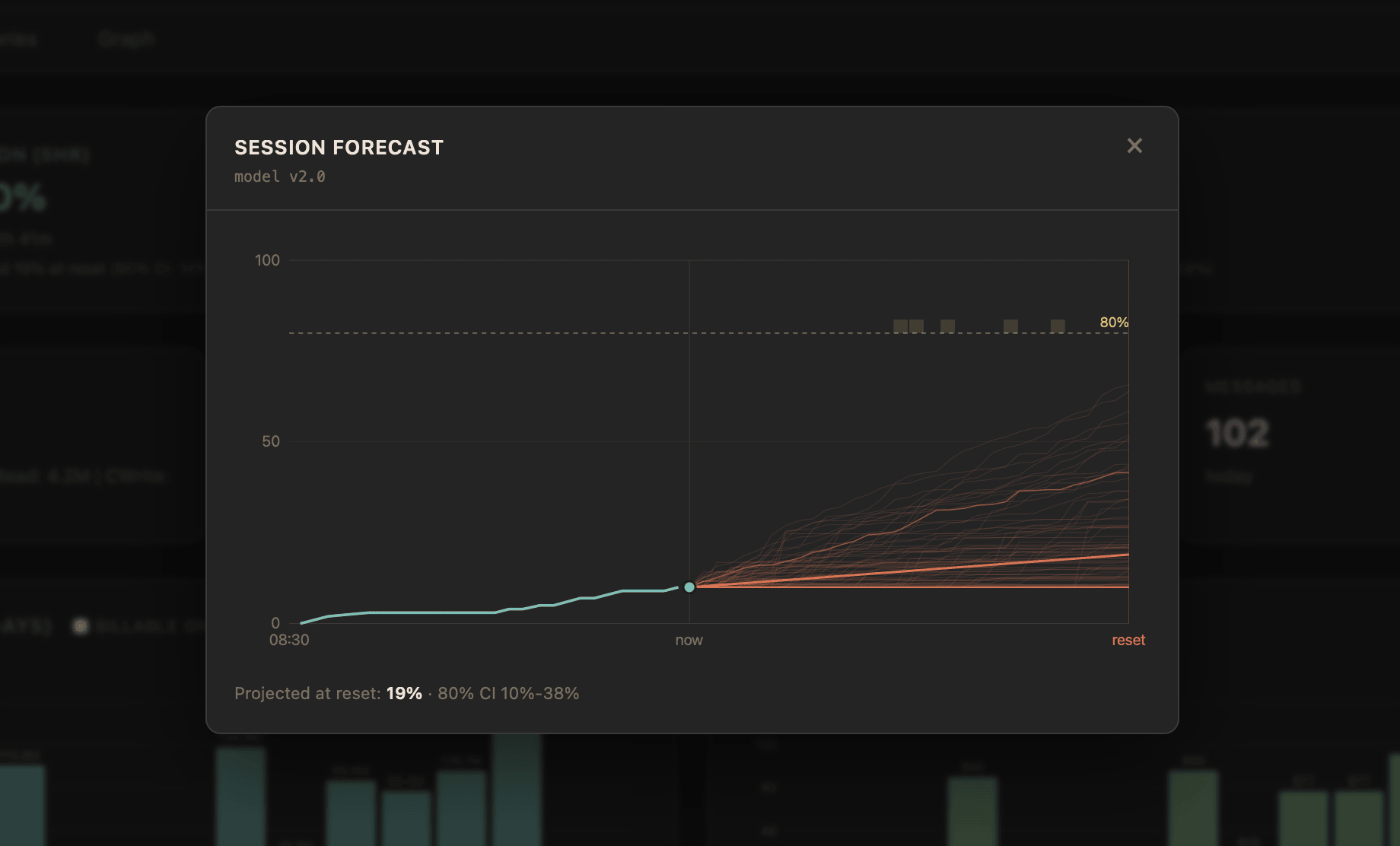
claumon session-window forecast showing projected utilization at reset with an 80% credible interval — The session-window forecast: projected utilization at reset with an 80% credible interval.

The forecaster reads utilization snapshots from the Claude OAuth usage API for each open rate-limit window (session, weekly, per-model weekly). For each gauge, it estimates demand at reset with an 80% credible interval, plus a median ETA to a threshold when more than half the simulated paths reach it before reset.

The design goal is to show uncertainty alongside the forecast. A flat recent gauge does not mean future usage is certain to stay flat; the model needs to allow both continued inactivity and renewed usage.

The model

This explanation follows model v2.2, released July 30, 2026. Four pieces carry the forecast. The derivation, calibration, and a worked example live in the v2.2 spec.

The path law. Inside the open window, projected demand accumulates as a Gamma process, a non-decreasing jump process. Conditioned on a positive rate $r$ , the increment over a horizon $s$ is

u (t_{now} + s) - u_{now} \sim Gamma (shape = \frac{r^{2} s}{σ_{session}^{2}}, scale = \frac{σ_{session}^{2}}{r})

so its mean and variance grow linearly in time:

𝔼 [u (t_{now} + s) - u_{now}] = r s, Var [u (t_{now} + s) - u_{now}] = σ_{session}^{2} s

Every increment is non-negative, so simulated paths are monotone and floored at the value now. A path whose sampled rate is exactly zero stays flat; the Gamma formula above applies to positive rates.

The rate, by empirical Bayes. The unknown rate $r$ combines the recent OLS slope ( $r_{OLS}$ , with standard error ${SE}_{OLS}$ ) and a prior fit on past sessions (mean $μ_{0}$ , variance $τ_{0}^{2}$ ) through a normal-normal conjugate update:

\frac{1}{τ_{post}^{2}} = \frac{1}{τ_{0}^{2}} + \frac{1}{{SE}_{OLS}^{2}}, r_{post} = τ_{post}^{2} (\frac{μ_{0}}{τ_{0}^{2}} + \frac{r_{OLS}}{{SE}_{OLS}^{2}})

The prior dominates early, when the slope is noisy; the data takes over as snapshots accumulate. The prior and calibration are refit daily from usage history.

For each simulated path, v2.2 draws a Gaussian rate using the posterior estimate and a variance floored by historical calibration, then maps negative draws to zero:

z_{k} \sim N (r_{post}, τ_{eff}^{2}), r_{k} = \max (0, z_{k})

Here $τ_{eff}^{2} = \max (τ_{post}^{2}, {\overline{τ}}^{2})$ , where the historical floor allows for changes in pace beyond the recent slope. This is a rectified Gaussian: negative draws become exactly zero, preserving a probability of no further growth. Positive draws drive the Gamma increments above.

This rate draw fixes a failure in v2.0 and v2.1. They sampled rates from a Gamma distribution matched to the estimated mean and variance. When the recent gauge plateaued, the estimated rate could approach zero while uncertainty remained substantial. In practice, the sampler then produced flat paths and intervals such as “80% CI 49%–49%.” In v2.2, some paths remain flat while others grow, so a plateau no longer erases the uncertainty.

The forecast and its spread. The point forecast extrapolates the posterior rate to reset,

F = u_{now} + r_{post} Δ t_{rem}

The implementation also retains an analytic spread summary, separating rate uncertainty (quadratic in the remaining horizon) from path noise (linear in it):

σ_{F}^{2} = \underset{rate uncertainty}{\underset{⏟}{Δ t_{rem}^{2} \max (τ_{post}^{2}, {\overline{τ}}^{2})}} + \underset{path noise}{\underset{⏟}{Δ t_{rem} σ_{session}^{2}}}

The retained analytic spread summary has two pieces: path noise grows linearly with the time to reset and dominates near reset, while rate uncertainty grows quadratically and takes over at longer horizons. The marked point is where they contribute equally.

These are retained analytic summaries. Rectifying the rate changes its moments, so the point forecast and spread above should not be read as the exact mean and variance of the v2.2 simulated distribution. The displayed 80% interval comes directly from the 10th and 90th percentiles of the Monte Carlo terminal values, including the flat paths.

Both interval edges and the point forecast can exceed 100%. They measure projected demand beyond the available quota; only the gauge ring saturates at 100%. A projection of 160% conveys how far demand could overshoot the limit.

The ETA. Because the paths are monotone, a threshold $C_{thr}$ is crossed once and stays crossed, so the first-passage time is well defined:

T^{*} = \inf {t > t_{now} : u (t) \geq C_{thr}}

Extrapolating the posterior rate gives a deterministic reference time,

{\tilde{T}}^{*} = t_{now} + \frac{C_{thr} - u_{now}}{r_{post}}

defined when the posterior rate is positive and the crossing falls before reset. The reported median ETA comes from the same Monte Carlo used for the forecast interval. Paths that do not reach the threshold before reset count as an infinite crossing time within this window.

The fraction of paths that never cross determines what can be reported:

50% or more: no median ETA is reported.
10% to less than 50%: a median and lower bound are reported, with an open-ended upper bound.
Less than 10%: a median and both interval bounds are reported.

The median accounts for all paths, including those that never cross. The implementation takes the interval bounds from the 10th and 90th percentiles of the finite crossing times, omitting the upper bound in the open-ended case.

Calibration and limits

The model is evaluated on held-out usage windows, checking interval coverage and scoring the predictive distribution with CRPS and quantile loss. The v2.2 changelog reports session coverage improving from 55% to 89% for the nominal 80% interval on its real-data benchmark, with a small improvement in CRPS. That is evidence from those exports, not a guarantee for every usage pattern.

The rate is still held constant within each simulated path. An abrupt change from active work to a long idle period can leave the forecast too high; renewed bursts can outpace it. The zero-rate probability helps represent abandoned sessions, but it does not model every change of pace within a window. With too little history, the forecaster waits for more data.

The repository maintains a versioned spec and archives retired versions. This page and its downloadable PDF describe v2.2.

View on GitHub · Download the v2.2 spec (PDF)